Space-time hotspots: how to unlock a new dimension of insights

You may have heard the statistic that 80% of data has a spatial component, and you can be sure that close to 100% has a temporal dimension. But how can you effectively analyze the interplay between the two?

Space-time clustering is one such approach.

This technique analyzes both spatial and temporal patterns, enabling businesses to unearth hidden trends and make more informed decisions at a granular level - both in space and time.

But how does it work, and how can you use it in your organization to drive better decision making? Keep reading to find out and follow our step-by-step guide to utilizing this approach to generate powerful business insights - fast!

What is Space-time clustering?

Imagine you’re an analyst at a food delivery company. Your job? To optimize deliveries. To do that, you’d need to know which locations have a high number of deliveries - i.e. where are the clusters or hotspots - so you can locate delivery drivers accordingly. Straightforward - right?

But hold on. There are clusters in three main locations; the central business district, a nightlife hotspot and a residential area. These locations are likely to have varying demand levels at different times of the day. Simply dispatching more delivery drivers across all of these locations would lead to a lot of wasted time - and therefore money.

This is the perfect use case for space-time clustering. This approach tells you not just where hotspots are, but where and when they are. This information allows you to add that extra dimension of insight to your decision making, crucial when profit margins are slim.

How does Space-time clustering work?

First of all, let’s talk about what a cluster or hotspot is.

Hotspot analysis identifies and measures the strength of spatial patterns by taking the user-defined neighborhood for each feature in a spatial table and calculating whether the values within that neighborhood are significantly higher or lower than across the entire table. There are a range of different hotspot algorithms available, with the two most common being the statistical tools Getis-Ord* vs Moran’s I; you can learn more about these in our full guide to spatial hotspots her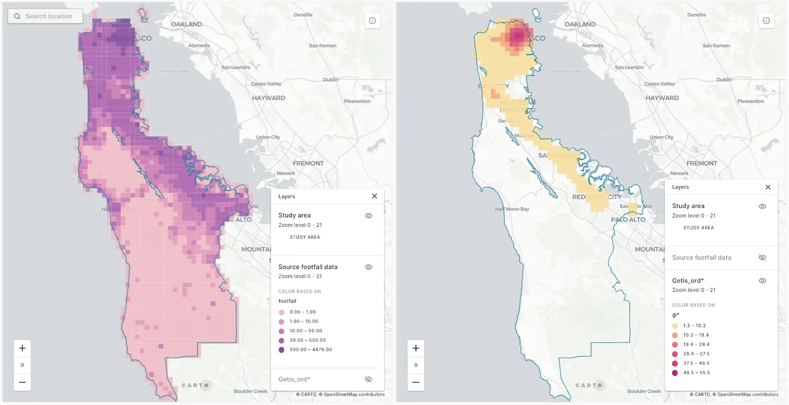e. Raw footfall count data (left) vs Getis-Ord hotspots (right).* Space-time clustering works in much the same way, but also assesses whether values are statistically significant over time, as well as space.

Our Analytics Toolbox for Google BigQuery includes functions that do just that by calculating the spatio-temporal Getis-Ord Gi* (GI*) statistic. Positive GI* values indicate that the neighborhood values are significantly higher than across the entire table - i.e. it is a hotspot - and negative GI* values indicate the reverse. You can read more about how this is calculated in our documentation.

Does this sound like something you need? Read on for a step-by-step tutorial!

Space-time clustering: a step-by-step guide

To follow along with this guide, you will need two things. First, a CARTO account; you can sign up for a free 14-day trial here if you don’t have one already.

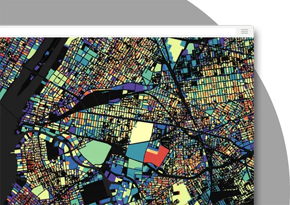
Secondly, you’ll need a dataset which you want to investigate! Any dataset with both space and time dimensions will work. In this example, we’ll be looking at spatial-temporal trends in the 1.8 million vehicle collisions which occurred in New York City from 2012-present (visualized in the map below, or open in full screen here). We’ll be investigating whether certain parts of the city experience more vehicle collisions at certain times of the day. This example is helpful for use cases such as transport planning or urban design.

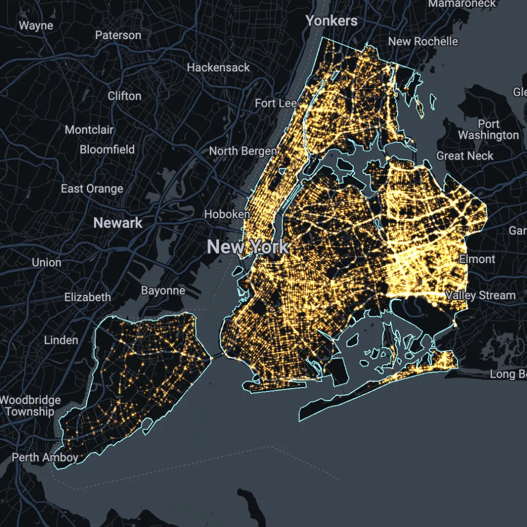[](https://clausa.app.carto.com/map/76f451d2-2c7f-4dc6-9888-72aebda03df6) If you’d like to follow along with this example, you can access the data [here](https://data.cityofnewyork.us/Public-Safety/Motor-Vehicle-Collisions-Crashes/h9gi-nx95). [](../workflows@utm_source=blog&utm_medium=website&utm_campaign=banner_workflows.html) ### Step 1: Data pre-processing

First of all, if your data isn’t already in the cloud, then you’ll need to load it to your Google BigQuery project, which you can do following this guide. If you don’t have access to your own project, you can use the CARTO Data Warehouse which is provided for all users.

Secondly, we need to make sure that our data is structured correctly to run this analysis. We’ll use the Spatial SQL below to do this, which will result in the following variables:

• A Spatial Index variable: the clustering technique we’ll be using requires data to be in a Spatial Index format i.e. a continuous spatial grid. To do this, in step 1 we’ll create a point geometry from the data’s longitude and latitude (ST_Geogpoint) and then in step 2 convert this to a H3 index (H3_FromGeogPoint). You can learn more about Spatial Indexes in this FREE ebook!-A timestamp: the collision time is originally stored in the variable “crash_time” as a string, so we’ll use a combination of string functions to access the hour value from this in step 1. Then, in step 2 we’ll convert this to a datetime variable type (DATETIME). We’ll assign “dummy” date and minute values as we want overall hourly values across the entire dataset.- ‍Collision count: calculated in step 2 using the COUNT() function. This could be replaced by any numeric variable which you want to calculate hotspots from.

WITH –Step 1: Create a point geometry and extract the hour field from the data collisions AS ( SELECT ST_GEOGPOINT(longitude, latitude) AS geom, CASE WHEN LENGTH(crash_time) = 5 THEN CAST(LEFT(crash_time,2) AS INT64) ELSE CAST(LEFT(crash_time,1) AS INT64) END AS hour FROM yourproject.yourdataset.newyork_collisions)

–Step 2: Convert to a H3 Spatial Index, count the collisions per hour/per cell, and create a timestamp SELECT carto-un.carto.H3_FROMGEOGPOINT(geom, 9) AS h3, COUNT(hour) AS collision_count, DATETIME(2023, 1, 1, hour, 0, 0) AS time FROM collisions GROUP BY hour, h3

Check out the results of this in the map below, or open in full screen here.

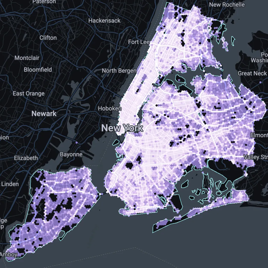[](https://clausa.app.carto.com/map/9aa9105a-dfc0-403e-9aa3-0cb69a04149b) ### Step 2: Running Space-Time Clusters

In this next step, we’ll run the Getis Ord SpaceTime function, available via our Analytics Toolbox’s statistics module for both H3 and Quadbin.

SELECT * FROM carto-un.carto.GETIS_ORD_SPACETIME_H3(( SELECT ARRAY_AGG(STRUCT(h3, time, collision_count)) AS input_data FROM yourproject.yourdataset.input_data ), 3, ‘HOUR’, 1, ’triangular’, ’triangular’);

Adapt the input query based on the data you prepared in step 1, then select your hotspot parameters:

• Neighborhood Size which will be taken into account to compute the Gi* value (here we use 3); this is measured in K-rings. A k-ring value of 1 includes the 6 cells (or 8 for a Quadbin index) which immediately border that cell. A value of 2 includes the cells which border those immediate cells, and so on.- Time unit is the time unit used. You can choose from the options year, quarter, month, week, day, hour, minute, or second. -Time interval is the number of adjacent intervals in time domain to be taken into account to compute the Gi* value, measured in the specified time units. Here, we are using 1 hour.- The Kernel function describes the spatial weights given to cells across the k-ring; you can define how much their proximity to the input cell affects the outcome of the analysis. Here we use triangular, which means cells further from the central cell have a much lower weight. Other options include uniform, triangular, quadratic, quartic, or gaussian.-The Time Kernel is similar, but applies to temporal weights. For more information, check out the full documentation for this function here.

Step 3: Interpreting the results

The output of step 2 will be a query including the index (H3/Quadbin) ID, the date/time, p value and GI*. At this stage, we recommend committing this query to a table.

The P value is the significance value which may allow us to reject the null hypothesis of our analysis. So if our null hypothesis was “there is no spatio-temporal clustering of collisions” then where cells fall under a set threshold, we can reject this. Typically, that threshold will be 0.01 or 0.05, associated with a confidence level of 99% or 95% respectively.

TheGI* value indicates the strength of clustering. Positive values indicate a strong spatial clustering of positive values relative to the wider dataset, while negative values indicate the reverse.

So, if we were interested in mapping statistically significant clusters of high values, we would want to run the following:

SELECT * FROM yourproject.yourdataset.youroutputtable WHERE p_value < = 0.05 AND GI > 0

The results? Check them out below!

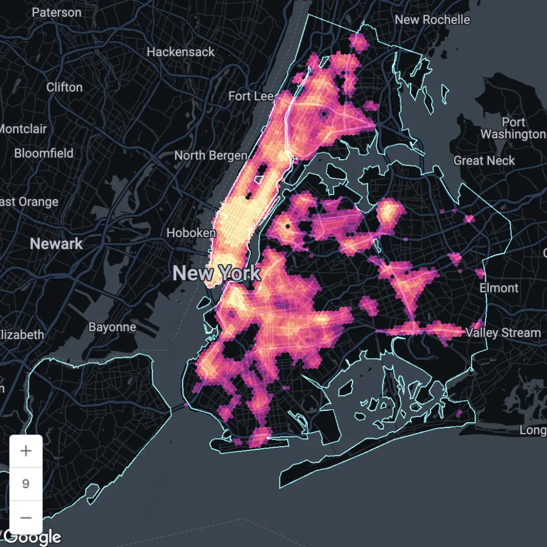[](https://clausa.app.carto.com/map/13ab912b-caf8-4916-8b60-6d614fdb5a00) Open in full screen [here](https://clausa.app.carto.com/map/13ab912b-caf8-4916-8b60-6d614fdb5a00).

We’ve made this visualization extra user-friendly and interactive by incorporating SQL Parameters. These allow you to add placeholders into your SQL (see below: {{time_from}} and {{time_to}}) to allow end users to interact with your data in a controlled way. Here, they are able to view the average GI* value over a specific time period - perhaps rush hour or late at night.

SELECT INDEX AS h3, *, EXTRACT(hour FROM date) AS hour FROM yourproject.yourdataset.youroutputtable WHERE p_value < = 0.1 AND gi > = 0 AND (EXTRACT(hour FROM date) > = {{time_from}} AND EXTRACT(hour FROM date) < = {{time_to}})

Space-time clustering for data-driven decision making

Space-time clustering is a game-changer for businesses seeking to extract actionable insights from their data. By examining both spatial and temporal dimensions, you can uncover trends, optimize operations, and make more informed decisions that drive growth.

Sign up for a free 14-day trial with CARTO today and start your Location Intelligence journey today!

Want to get started? [

Start free trial

](https://app.carto.com/signup/)

This article was developed as part of the EMERALDS project, funded by the Horizon Europe R&I program under GA No. 101093051.

Don’t forget to share this post on Linkedin!